
Dave Adams
Sky Television, UK
Many people have written about using a CDM chart to obtain an optimised matrix for their camera. In a moment I will discuss the best technique that I believe enables you to do this, but let’s first take a moment to think about why we might want to optimise our matrix.
If a CDM chart is to be trusted then the colours it displays once viewed through a correctly white-balanced camera, should appear at certain pre-determined points on the vectorscope under ITU-709 recommendations. Not all cameras do this but the reason we might want to do this is with the aim of reproducing the scene as realistically as possible. As an engineer this should be your first starting point before building any custom look.
First of all we must banish the use of any multi-matrix or colour corrector from the optimisation process as they are non-linear tools. The linear-matrix is what effects the RGB response curves. This technique has been designed to be repeatable in any controlled environment without the need for laboratory conditions – a dark room with a single black-body light source is ideal.
Any CDM chart with at least 24 colours will enable you to optimise your matrix, although the more colours the better. The Harlequin chart is ideal for custom matrix building – with over 170 precision colours you can see with even greater detail as to how you are adjusting the colour-space.
There are two important things to bear in mind: 1) Linearity is key; and 2) Throw away the vectorscope. Luminance cannot be viewed on a vectorscope but can be on a waveform monitor, along with hue and saturation. Instead, use the vectorscope at the end to check your results.
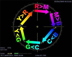 Working with the colour-space as a whole is near-impossible. The best method is to divide the colour space into six sectors, each comprising of a primary colour, a secondary colour, and all in between [Figure 1]. You can now build six individually-optimised matrices; one for each sector.
If each sector given above is in turn displayed at line rate, then the waveform monitor will show two horizontal lines when looking at the most saturated colours – in this instance one at 551 mV, the other at 289 mV – and a third which steps between the two.
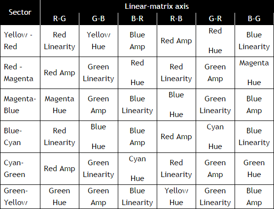
View the two linear [i.e. un-stepped] channels for any given sector in RGB overlay on a waveform monitor and the optimisation process can begin. One of the six axes of the linear-matrix will change the amplitude of one colour channel, and a second will linearise it. The third and fourth axes provide the same functions for the other linear channel. The fifth and sixth axes change the hue of the primary and secondary colours; however this can introduce coefficients that have a negative impact once the results are averaged so generally little adjustment is made. [Table 1].
Table 1 – Adjustments Through the Linear Matrix
Averaging these results for all the sectors creates a ‘first compromise’ matrix. The results from all six sectors are tabulated and shown in Table 2. [These values have been disguised and are not intended to be representative of any camera].
Table 2 – Matrix Adjusted Results
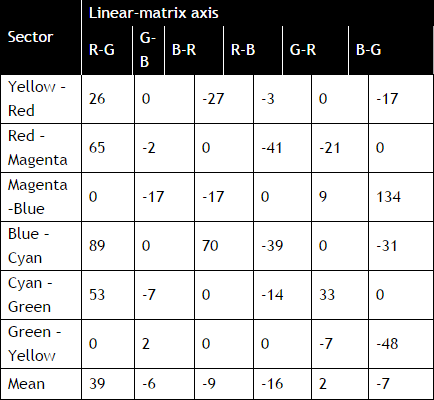
Some of these coefficients are rather large. Large weightings are required to achieve the best results for individual sectors, but once averaged they distort the other sectors too much.
A coefficient of ‘68’ is where abnormalities tend to start occurring on this example. Trial and error proved that a capping value of ‘51’ gave the best results overall. Shown in Table 3 are the new results after the artificial cap has been applied.
Table 3 – Matrix adjustment results – capped
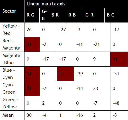
The coefficients in Table 3 now provide a compromise for the colour-space at large, but they are not necessarily the best for skin tones. In this example, one final adjustment to B-G is made on their behalf to complete the optimization process. [Table 4].
Table 4 – Matrix adjustment results

To summarise the process, compare Figures 2-5 taking into account RGB linearity, signal-to-noise, vectorscope phase and ‘dot’ irregularity.
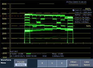
Figure 2 – HD Camera with no matrix adjustments
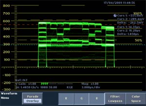
Figure 3 – Matrix adjusted using linearization technique
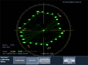
Figure 4– HD Camera with no matrix adjustments
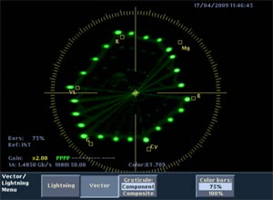
Figure 5 – Matrix adjusted using linearization technique
Your camera will now reproduce the scene as realistically as possible and you are now in a good position to build your own custom look by modifying your results or this technique.
This TechTip has been adapted from the paper Selecting Production Parameters to Ensure that Picture Quality Accommodates the Intended and Possible Future Imaging Systems which was presented at the SMPTE Tech Conference in Hollywood, CA, 27th October 2009.

